Diffusion models — Langevin & SDE

Introduction

There are basically some sections i want to connect & establish a link btw them. First of them being langevin diffusion, see diffusion model rely on Stochastic differential equations & langevin is a specific SDE which is fundamental to understand diffusion. Another one is Ito-SDE we’ll cover it too.

Langevin Diffusion

What is Langevin Diffusion?

Langevin diffusion has been discovered in physics to describe the motion of particles driven by random and deterministic forces. Due to the random forces, it is a stochastic process that in generative AI describes the evolution of a probability distribution over time.

Langevin diffusion is often used as a way to sample from a probability distribution p(x). Think of p(x) as a very complex high dimensional distribution that represents a dataset.

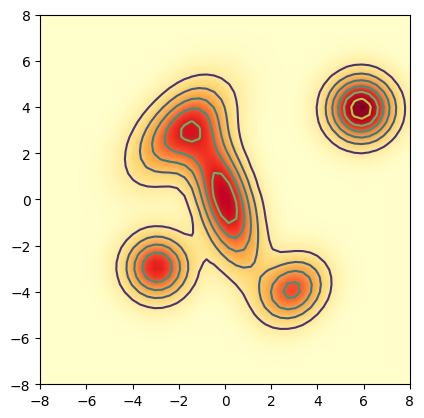
Gaussian mixture is given by a weighted sum of Gaussian distributions:

$$ p(\mathbf{x}) = \sum\limits_{j=1}^{n}q_j \mathcal{N}(\mathbf{x};\mu_i,\Sigma_{i}), \quad \text{where } q_j\in\mathbb{R},\sum\limits_{j=1}^{n}q_j = 1,\mu_i\in\mathbb{R}^2,\Sigma_{i}\in\mathbb{R}^{2\times 2} $$

namely the density, log-density, score (`gradient of log_density`), and gradient of the density.

$$ \begin{aligned} \mathcal{N}(x;\mu,\Sigma) &= \frac{1}{(2\pi)^{d/2}|\Sigma|^{1/2}} \exp\!\left(-\frac{1}{2}(x-\mu)^\top \Sigma^{-1}(x-\mu)\right), \\[6pt] \log \mathcal{N}(x;\mu,\Sigma) &= -\frac{d}{2}\log(2\pi) - \frac{1}{2}\log|\Sigma| - \frac{1}{2}(x-\mu)^\top \Sigma^{-1}(x-\mu), \\[6pt] \nabla_x \log \mathcal{N}(x;\mu,\Sigma) &= -\Sigma^{-1}(x-\mu), \\[6pt] \nabla_x \mathcal{N}(x;\mu,\Sigma) &= -\mathcal{N}(x;\mu,\Sigma)\,\Sigma^{-1}(x-\mu). \end{aligned} $$

Score Function & Vector Fields

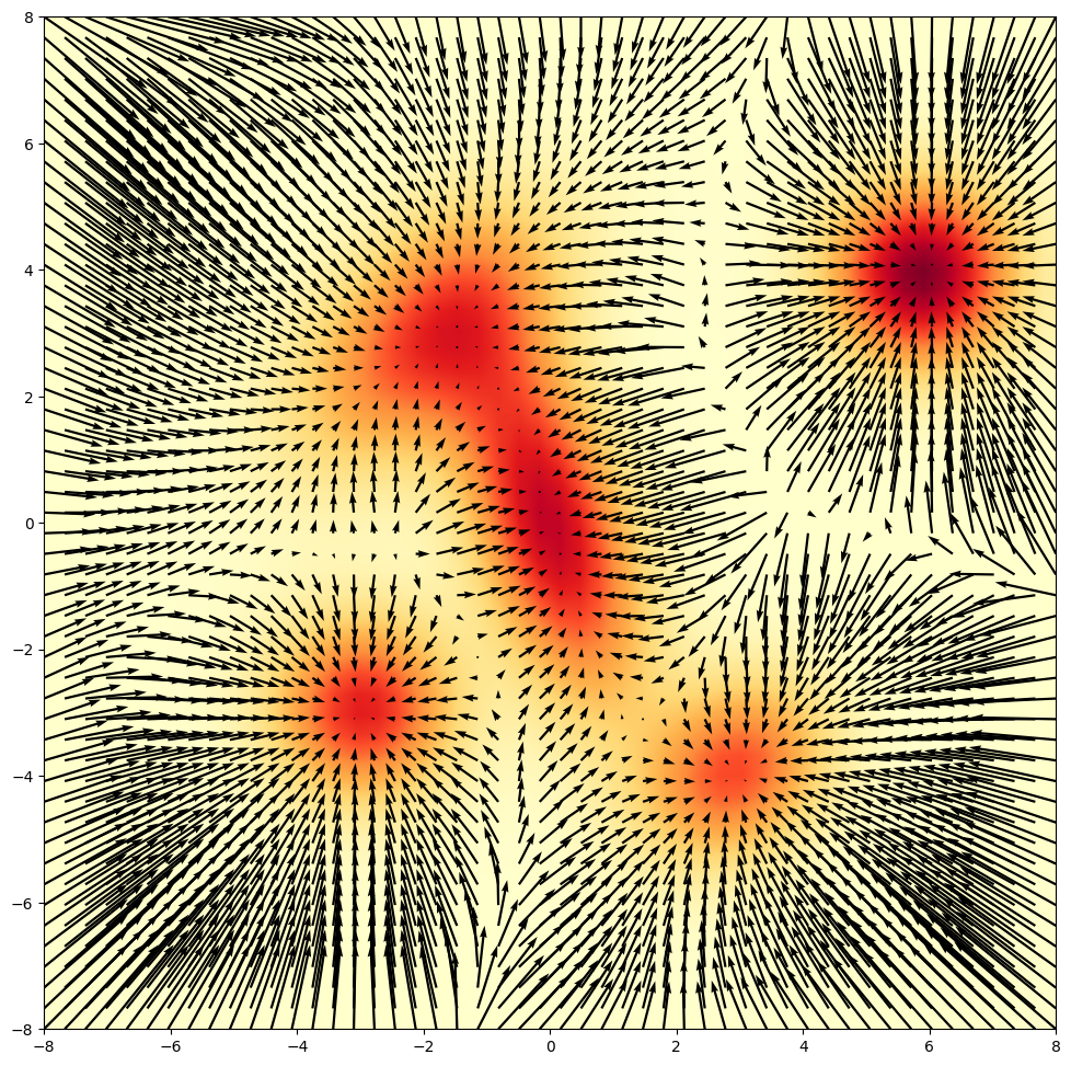
Now in p(x) peaks are high-probability data (like clear images of cats) and the valleys are low-probability noise, the gradient of p(x) acts like a compass. So we use the score to "push" random noise toward the data peaks basically gradient ascent. This process is called Langevin dynamics. Why log is just mathematical convenience cause prob at points might be very low like in orders of -50 then that exponential term removal & since logarithm is a monotonically increasing function. This means that the peak of p(x) is in the exact same location as the peak of log p(x).

When you combine them, the score function creates a vector field.

$$ \nabla_x \log p(x) = \frac{\nabla_x p(x)}{p(x)} $$

Langevin Diffusion describes a Stochastic Differential Equation, i.e. the evolution of random variable or like particle X at time t (X_t) over time t & here W_t is brownian motion, s is the step size

$$ dX_t = \nabla\log p(X_t) + \sqrt{2}W_t $$

$$ X_{t+s} = X_{t}+s\nabla\log p(X_{t})+\sqrt{2s}\epsilon, \quad \epsilon\sim\mathcal{N}(0,\mathbf{I}_d) $$

In other words, the update of the step of X_t is performed by Going into the direction of the gradient & Adding some random Gaussian noise.

Intuitively, the Langevin diffusion is gradient ascent maximing the log-probability injected with random Gaussian noise.

Now the main thing is that actually we don’t know gradient for the clean data so now we’ll train a neural network (the Score Estimator) to predict the gradient of the noisy data. As the noise level drops to zero, the network's "push" becomes more refined, eventually guiding the noise into a perfect sample from the true distribution p(x). This is more in future where in forward pass add noise & then in reward pass our network will try to predict that score / noise which is like gradient ascent.

Ito SDEs & Stochastic Processes

What the hell is this ItoSDE??

SDE describes how one particle moves, if you simulate 10,000 particles at once, the density of where those particles end up will eventually match the probability distribution p(x) perfectly. How does density comes into play?? now think of this at macroscopic level: all the particles follow the same compass and the same rules of random walking, they will eventually cluster in certain areas. The density is simply the "heatmap" of where all those millions of particles are at time t.

Analogy: Think of a drop of ink in water. The SDE describes the chaotic path of a single molecule of ink. But when you look at the whole glass, you see the ink spreading out into a smooth, predictable cloud.

So the beauty of stochastic processes comes in studying how X_t+s is related to X_t for a single random particle X. A fundamental stochastic process is a Brownian motion W_t. There is a famous partial differential equation (PDE) called the Fokker-Planck Equation. It describes how the density of a crowd of particles changes over time if every individual particle is following the SDE above.

$$ W_{t+s} = W_{t} +\sqrt{s} \epsilon\quad\text{where }\epsilon\sim\mathcal{N}(0,1) $$

A Stochastic Differential Equation "is an Ordinary DE but just random".

$$ \frac{d}{dt}\mathbf{x}(t) = f(\mathbf{x}(t),t)\\[6pt] dX(t) = f(X_t,t)dt+g(t)dW_t $$

Now in the SDE a deterministic drift specified by a function f & random drift specified by a function g.

$$ X_{t+s}\approx X_{t}+s f(X_t,t)+g(t)\sqrt{s}(W_{t+s}-W_{t})\\[6pt] X_{t+s} = X_{t} + sf(X_{t},t)+g(t)\sqrt{s}\epsilon\\[6pt] X_{t+s}|X_t\sim\mathcal{N}(X_{t}+s f(X_t,t),sg^2(t)) $$

so here the mean is shifting towards the deterministic function & variance is by random drift function.

So the deterministic drift f describes the infinitesimal change in mean and the volatility function g describes the infinitesimal standard deviation.

Now the imp questions are

1. Can we say something about the expectation value or mean E[X_t]?
2. Can we say something about the variance V[X_t]?
3. Can we say something about the distribution X_t∼pt?

In general, the distribution of X_t can be relatively complex.

In order to to be able say more, we have to make the following assumption of affine drift coefficients. We assume that f has an affine form, i.e.

$$ f(x,t)=a(t)x+b(t)\\[6pt] X_{t+s}-X_{t}\approx sa(t)X_t+sb(t)+g(t)\sqrt{s}\epsilon \\[6pt] X_{t}|X_0 \sim\mathcal{N}(\mathbb{E}[X_t|X_0],\mathbb{V}[X_t|X_0]) $$

And if you’re curious why affine coefficients basically they help us to calculate the Expectation & variance. something like this & same there is for variance

$$ \begin{align*} \mathbb{E}[X_t|X_0]&=\left(X_0+\int\limits_{0}^{t}\exp(-\int\limits_{0}^{s}a(r)dr)b(s)ds\right)\exp\left(\int\limits_{0}^{t}a(s)ds\right)\\ \mathbb{E}[X_t]&=\left(\mathbb{E}[X_0]+\int\limits_{0}^{t}\exp(-\int\limits_{0}^{s}a(r)dr)b(s)ds\right)\exp\left(\int\limits_{0}^{t}a(s)ds\right) \end{align*} $$

SDE Frameworks for Diffusion

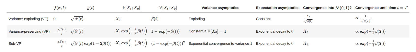
There are 3 frameworks to build SDEs for diffusion models: variance-preserving, variance sub-preserving and variance-exploding.

consider noise functions β(t) that satisfy:

1. β(0)=0
2. β′(t)≥0
3. β(t)→∞ for t→∞

This was for variance preserving, next one for variance exploding & then sub variance preserving:

$$ X_{t_{i+1}}=\sqrt{1-(\beta(t_{i+1})-\beta(t_i))}X_i+\sqrt{(\beta(t_{i+1})-\beta(t_i))}\epsilon\\[6pt] q(x_{t+h}|x_{t}) = N (x_{t+h}; x_{t},(\beta(t_{i+1})-\beta(t_i))\mathbb{1}) $$

Now in the variance exploding case see what happens to variance it won’t stop at 1 it will keep on inc but the mean value would be same as X_0.

$$ \mathbb{E}[X_t|X_0]=X_0, \quad \mathbb{E}[X_t]=\mathbb{E}[X_0] \\[6pt] \mathbb{V}[X_{t}|X_0] =\beta(t)\\ \mathbb{V}[X_{t}] =\mathbb{V}[X_0]+\beta(t) $$

Now this won’t converge as ofc variance is exploding but there is rescaled version which is just, now the mean remains same but the variance shrinks by factor of beta(t) which makes the variance equals 1. Without this scaling, your SDE is like a Standard Brownian Motion. If you let a particle wander forever, it will eventually wander to infinity. There is no "stationary distribution" because the particle just keeps getting further and further away. By rescaling to Y_t, you turn the process into something resembling an Ornstein-Uhlenbeck (OU) process.

$$ Y_t=\frac{X_t}{\sqrt{\beta(t)}} $$

Now the variance for sub-VP SDE is always smaller than the variance for the VP SDE.

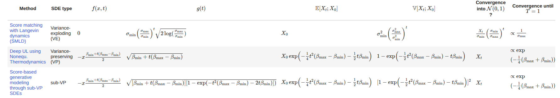
Now like we can keep it linear or exponential like in Generative Modeling by Estimating Gradients of the Data Distribution proposed to use a variance-exploding SDE from t=0 to t=T=1 such that the noise scales follow a geometric sequence from standard deviation σmin to σmax:

$$ \Rightarrow \sqrt{\beta(t)}=\sigma_{\text{min}}\left(\frac{\sigma_{\text{max}}}{\sigma_{\text{min}}}\right)^t $$

in DDPM it was proposed to use a model that corresponds to a variance-preserving SDE running from t0 to t=T=1 setting

$$ \beta(t)=\frac{1}{2}t^2(\beta_{\text{max}}-\beta_{\text{min}})+t\beta_{\text{min}} $$

the sub VP SDE also uses same beta(t)

So to give a flow first thing we define how X_t+1 will come up from X_t with B_t now since this would be gaussian we will calculate the expectation & variance. And expectation would relate to f(x, t) & variance with g(t). Now we will get affine coefficients from f(x, t) & hence will get close form equation for mean & variance.

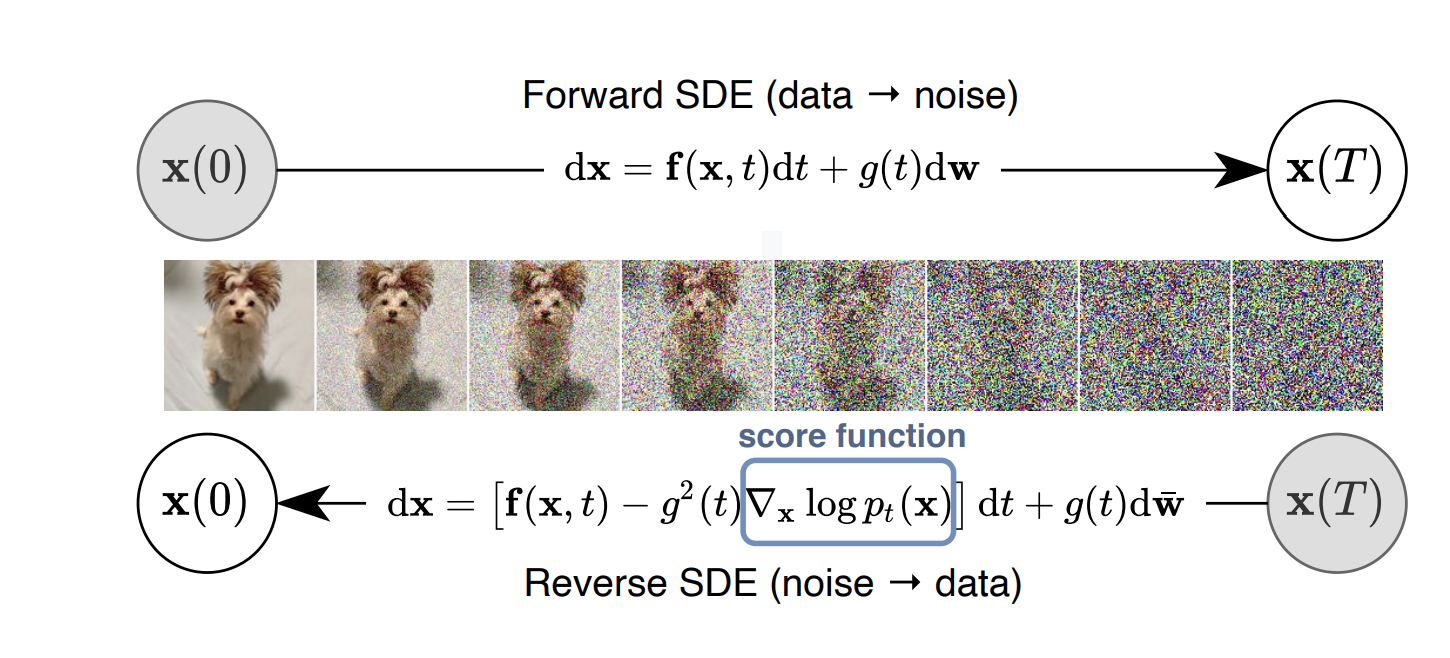
Reverse-Time SDE & Score Estimation

Now the main idea comes into play & that is like we can only sample the images that are in dataset with representation p_data but say they are just 10k now what. So see the idea is that noise or normal distribution is what we will sample from & then we’ll run a reverse SDE to reach X0 ∼ p_data.

So firstly equation for reverse time SDE is:

$$ d\bar{X}_t= \bar{f}(X_t,t)dt + \bar{g}(t)d\bar{W}_t\\[6pt] \bar{X}_{t-s}-\bar{X}_t \approx - s\bar{f}(\bar{X}_t,t)+\sqrt{s}\bar{g}(t)\epsilon \\[6pt] \bar{g}=g \\ \bar{f}(x,t)=f(x,t)-g^2(t)\frac{\partial}{\partial x}\log p_{t}(x)\\[6pt] d\bar{X}_t= [f(X_t,t)-g^2(t)\frac{\partial}{\partial x}\log p_{t}(\bar{X}_t)]dt + g(t)d\bar{W}_t\\[6pt] \bar{X}_{t-s} \approx \bar{X}_t +s\left[g^2(t)s_{\theta}(\bar{X}_t,t)-f(\bar{X}_t,t)\right]+\sqrt{s}g(t)\epsilon $$

where p_t(x) is the density of the distribution of X_t.

Now see here the f(x, t) is a pushing or contractive force that pulls towards the mean 0 in normal forward pass, so in reverse dynamics there is -f(x, t) that makes it act as expansive force with g(t) term that acts as anti-entropy cause it makes in direction of score.

these methods are called score-based generative models: to generate the reverse-time SDE, we "only" need to train a model to predict the score - everything else is defined by us.

$$ s_{\theta}(x,t)=\frac{\partial}{\partial x}\log p_t(x) $$

Reverse SDE is the continuous-time generalization of Annealed Langevin Dynamics. For the variance exploding SDE, we have that:

$$ \bar{X}_{t-s}\approx\bar{X}_t+h\frac{\partial}{\partial x}\log p_t(\bar{X}_t)+\sqrt{h}\epsilon\\[6pt] h=sg^2(t)\\[6pt] p_t(x_t)=\int \mathcal{N}(x_t;x_0,\beta(t))p_{\text{data}}(x_0)dx_0 $$

As noise decreases it goes to p_data. we anneal the distribution to the data distribution, The advantage of annealed Langevin dynamics is in regions of low probability p_data, we have very poor estimates of the scores (just out of data scarcity). Therefore, upon initialization, one uses a noised version (introducing bias to remove high variance).

Now for the loss part we can compute loss because it only depends on the conditional distribution which is normally distributed because we assumed affine drift coefficients, like we have shown above how we can get expectation & variance easily

$$ p_{t|0}(x_t|x_0)=\mathcal{N}(x_t;\mathbb{E}[X_t|X_0=x_0];\mathbb{V}[X_t|X_0=x_0])\\[6pt] \frac{\partial}{\partial x_t}\log p_{t|0}(x_t|x_0)=-\frac{x_t-\mathbb{E}[X_t|X_0=x_0]}{\mathbb{V}[X_t|X_0=x_0]} $$

and we can use this score network as a denoising network

$$ \epsilon_{\theta}(x_t,t)=-s_{\theta}(x_t,t)\sqrt{\mathbb{V}[X_t|X_0=x_0]}\\ s_{\theta}(x_t,t)=-\frac{\epsilon_\theta(x_t,t)}{\sqrt{\mathbb{V}[X_t|X_0=x_0]}}\\[6pt] x_t=\sqrt{\mathbb{V}[X_t|X_0=x_0]}\epsilon+\mathbb{E}[X_t|X_0] $$

Fokker-Planck & Probability Flow

Wait, why Fokker-Planck?

Think of the Score as a Force Field.

- The SDE view: You are a leaf being blown by a fan (the Score) while also being hit by random raindrops (the Noise). Your path is chaotic.
- The ODE (FPE) view: You are a drop of water in a pipe. The "pressure" in the pipe is determined by the Score. You just flow smoothly from high pressure to low pressure.

Even though the "Fan" and the "Pressure" are both derived from the same Score Function, the way the particle moves is fundamentally different.

$$ d\bar{X}_t= [f(X_t,t)-g^2(t)\nabla\log p_{t}(\bar{X}_t)]dt + g(t)d\bar{W}_t \\[6pt] d\bar{X}_t= [f(X_t,t)-\frac{1}{2}g^2(t)\nabla\log p_{t}(\bar{X}_t)]dt $$

-f(x, t): acts like an expansion force. It "un-shrinks" the image, pulling it back out from the zero-center.

-g^2(t)*score: This is the Guided Force. It uses the "volume" of g(t) to steer the particle. It's the only force that actually knows the difference between a cat and a dog. It fights the randomness to find the features.

g(t)dW_t: (In the SDE version) provides a little bit of "vibration" to make sure the particle doesn't get stuck and explores the whole shape of the cat correctly.

The Deterministic ODE (No Jitter): The gradient (score) will point to the closest peak. The particle will slide into that one peak. This is called Mode Collapse.

The Stochastic SDE (With Jitter): The dW_t term provides kick. This jitter allows the particles to explore the whole landscape and represent the entire distribution p(x), not just the local maxima.

Deterministic ODE Sampling

Now then how do we add randomness in ODE, its basically deterministic so initial noise vector X_t is like picked randomly as starting point in a massive high-dimensional Gaussian space. By picking a different X_t, you are "exploring" the different outcomes.

$$ \bar{X}_{t-s} \approx \bar{X}_t +s\left[g^2(t)s_{\theta}(\bar{X}_t,t)-f(\bar{X}_t,t)\right]+\sqrt{s}g(t)\epsilon \\[6pt] \bar{X}_{t-s} \approx \bar{X}_{t} + s\left[\frac{1}{2} g^2(t)\,\theta(\bar{X}_{t},t) - f(\bar{X}_{t},t)\right] $$

Now how does the picture of big steps come into play see first of all the step term is in the score & the noise (epsilon) term as well. So if the step becomes big then the chaos or noise also goes big but in case of ODE even if we increase the step size it is just with score so nothing chaotic happens.

See the score is basically our guiding force & think of g(t) as just temperature like how strong that force is then -f(x, t) is expansive force & then there is epsilon noise. So in SDE if step size is 0.001 then noise ~0.03. Now say we took step size as 0.05 so noise ~0.22 which is huge. A single kick of 0.22 is a massive jump in pixel-space. If the model makes a mistake in the Score at that moment, the giant noise kick will throw the particle into a forbidden zone which is why ODEs are preferred.

Now in training noise is used but sampling/generation is the game where if noise if used(DDPM) if not (DDIM).

Consistency Models

Consistency models as the name suggests is consistent that means whatever be the input the output would always be clean image normally that is $x_0$ but here shown as $x_\epsilon$.

For any two time points $t$ & $t'$ on the same trajectory:

$$f(x_t,t)=f(x_{t'},t')= x_\epsilon$$

There are two ways to train a consistency model: consistency distillation (CD) and consistency training (CT).

Consistency Distillation (CD)

In consistency distillation, you already have a trained diffusion model (the “teacher”). You use it to generate a trajectory. The loss is basically the distance between the output of the target consistency model using a one-step diffusion generated image at $t_n$ with the consistency model output using $x_{t_{n+1}}$.

So $x_{t_{n+1}}$ is a noisier sample, and the diffusion model deterministically steps it to a slightly less noisy sample $x_{t_n}$ using something like the probability flow ODE.

You feed $x_{t_{n+1}}$ into the student consistency model $f_\theta(x_{t_{n+1}}, t_{n+1})$ and $x_{t_n}$ into a target (EMA) consistency model $f_{\theta^-}(x_{t_n}, t_n)$, then minimize the distance between those two outputs.

$$ \mathcal{L}^N_\text{CD} (\theta, \theta^-; \phi) = \mathbb{E} [\lambda(t_n)d(f_\theta(\mathbf{x}_{t_{n+1}}, t_{n+1}), f_{\theta^-}(\hat{\mathbf{x}}^\phi_{t_n}, t_n)] $$

Consistency Training (CT)

In consistency training, we don't have a pretrained score model, so we must estimate the score ourselves to define local trajectory structure.

They use the fact that if you take a clean image $x$ and add Gaussian noise $x_t = x + t z$ where $z \sim \mathcal{N}(0, I)$, then the score has a closed-form unbiased estimator:

$$\nabla \log p_t(x_t) \approx -(x_t - x) / t^2$$

CT loss is: $$ \mathcal{L}^N_\text{CT} (\theta, \theta^-; \phi) = \mathbb{E} [\lambda(t_n)d(f_\theta(\mathbf{x} + t_{n+1} \mathbf{z},\;t_{n+1}), f_{\theta^-}(\mathbf{x} + t_n \mathbf{z},\;t_n)] $$

Why ODE Solvers Matter?

To move from $t_{n+1}$ to $t_n$, you must numerically integrate the ODE. Since neural networks give you an approximate vector field, we need robust solvers.

Euler’s method uses the slope at the starting point and assumes it’s constant across the step. Heun’s method (second-order) takes an Euler step, evaluates the slope again there, and averages the two, better approximating the trajectory's curvature.

This matters because the entire training signal depends on the pair $(x_{t_{n+1}}, x_{t_n})$ lying on the same true probability flow trajectory.

Latent Diffusion Models (LDM)

Latent Diffusion Models (LDM) loosely decomposes the perceptual compression and semantic compression by first trimming off pixel-level redundancy with an autoencoder and then manipulating/generating semantic concepts with the diffusion process on the learned latent.

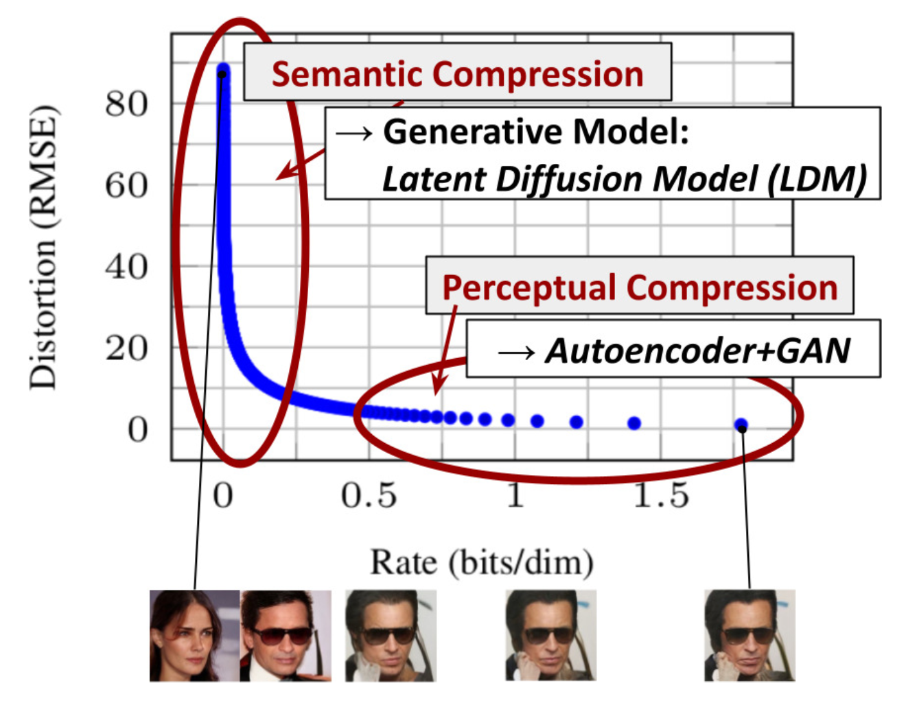
Distortion (RMSE) vs Rate (bits/dim) in Latent Space

On the vertical axis, you have distortion (RMSE). That’s just reconstruction error — how different the reconstructed image is from the original at the pixel level. Lower is better.

On the horizontal axis, you have rate in “bits per dimension” (bits/dim). This is a normalized compression measure: how many bits are used to encode each dimension. Low bits/dim means high compression.

On the left (very low rate), distortion explodes. This is where Semantic Compression happens. If you barely use any bits, reconstruction is poor, but the "meaning" can still be captured. On the right, distortion is low and decreases slowly, representing Perceptual Compression (via Autoencoder + GAN).

Perceptual vs Semantic Compression

Perceptual compression is about preserving how the image looks to us (textures, edges). It removes pixel redundancy. Semantic compression is more radical: it stores the meaning of the image and regenerates a plausible image from that meaning.

In LDM, the Autoencoder handles the perceptual part (removing redundancy), while Diffusion handles the semantic modeling (generating meaningful structure).

The latent $z$ is NOT just a flat vector. In Stable Diffusion, it's a 3D tensor ($H \times W \times C$). It behaves like a lower-resolution image with learned features.

Latent Space Regularization

Denoising in latent space is not just a cleanup step; it IS the generation process. Diffusion models learn to reverse a gradual noising process. It's like sculpting a statue by gradually removing randomness instead of adding clay.

To make training stable, we often use KL regularization. This encourages the encoder to make latents look roughly like samples from a standard normal distribution. If the latent space is wildly irregular, diffusion training becomes unstable. KL regularization smooths and shapes this space.

Cascaded Diffusion & Augmentation

Generating high-res images (e.g., $1024 \times 1024$) in one shot is computationally expensive. Cascaded Diffusion breaks this down:

• Stage 1: Generate a low-resolution image.
• Stage 2 & 3: Super-resolve the output of the previous stage.

Each stage conditions on the output of the previous one. However, generated images are imperfect. To make the super-res model robust, we use Conditioning Augmentation: intentionally corrupting the low-res input during training so the model learns to handle messy upstream outputs.

This can be Truncated (stopping the reverse process early) or Non-truncated (re-corrupting a clean sample with forward diffusion).

unCLIP (DALL-E 2)

unCLIP (the core of DALL-E 2) factorization: $$P(x | y) = P(x | c_i, y) \cdot P(c_i | y)$$

It splits the task into two parts:

• Prior: Predicts the CLIP image embedding $c_i$ from the text caption $y$. It generates a semantic vector, not pixels.
• Decoder: A diffusion model that generates the final image conditioned on that predicted CLIP image embedding.

Why split? Because CLIP embeddings are powerful semantic summaries. The prior models the semantic distribution, while the decoder models the perceptual image structure.